How to create a user in MySQL and grant a permission

In MySQL we can have multiple databases created which can be associated with some specific
functions. MySQL is the default database which is created while initial installation of the database. Using the following steps you will be able to create a user for a specific database and also if you want you can assign a password to it.

1. First of all create a user in the MySQL Database after log into it, using the following query:

mysql> CREATE USER 'abcd'@'localhost' IDENTIFIED BY '1qazXSW@';

2. Grant all or specific privileges to the new user and also assign a password as required.

mysql> GRANT ALL PRIVILEGES ON  abcd_designs.* TO 'abcd'@'localhost';

                                                                     or

mysql> GRANT SELECT, INSERT, UPDATE, DELETE, CREATE, DROP, ALTER, INDEX ON abcd-designs.* TO 'abcd'@'localhost'  IDENTIFIED BY 'abcd@123';

3. After performing all the above operations, in-order to tell the server to reload the grant tables, perform a flush-privileges operation. This can be done by issuing a FLUSH PRIVILEGES statement or by executing a mysqladmin flush-privileges or mysqladmin reload command.

A grant table reload affects privileges for each existing client connection as follows:

• Table and column privilege changes take effect with the client's next request.
• Database privilege changes take effect the next time the client executes a USE db_name statement.

Note:
Client applications may cache the database name; thus, this effect may not be visible to them without actually changing to a different database or flushing the privileges.

• Global privileges and passwords are unaffected for a connected client. These changes take effect only for subsequent connections.

If the server is started with the --skip-grant-tables option, it does not read the grant tables or implement any access control. Anyone can connect and do anything, which is insecure. To cause a server thus started to read the tables and enable access checking, flush the privileges.

mysql> FLUSH PRIVILEGES;

If there is a "-" hyphen between the names then we can use backtick to bypass it like `abcd-designs`

Attributes:

Database name = abcd_designs
User name = abcd
Password = abcd@123

Recover MySQL root Password

MySQL is an open-source relational database management system(RDBMS).MySQL is a central component of the LAMP open-source web application software stack (and other "AMP" stacks). LAMP is an acronym for "Linux, Apache, MySQL, Perl/PHP/Python". 

All My SQL databases on a server are always protected by a root password for better security. Server Administrator's have access to such information's for better troubleshooting of any issue. In case's where you forget the My SQL root password, you can use the following method to reset the My SQL root password.

# /etc/init.d/mysql stop 

# mysqld_safe --skip-grant-tables & 

# mysql -u root 

mysql> use mysql; 

mysql> update user set password=PASSWORD("NEW-ROOT-PASSWORD") where User='root'; 

mysql> flush privileges; 

mysql> quit
# /etc/init.d/mysql stop 

# /etc/init.d/mysql start 

# mysql -u root -p

How to replace MySQL with MariaDB in cpanel.

MariaDB is an enhanced drop-in replacement for MySQL. MySQL 5.1 is compatible with MariaDB 5.1, 5.2 and 5.3. MySQL 5.5 is compatible with MariaDB 5.5. 

• Make sure to save all existing data just in case there are any issues.     

cp -Rf /var/lib/mysql /var/lib/mysql-old 

mv /etc/my.cnf /etc/my.cnf-old  

• Disable all the targets so cPanel no longer handles MySQL updates. The following will mark the versions of MySQL we distribute as uninstalled so they are no longer maintained by cPanel/WHM:
  
  /scripts/update_local_rpm_versions –edit target_settings.MySQL50 uninstalled 

/scripts/update_local_rpm_versions –edit target_settings.MySQL51 uninstalled 

/scripts/update_local_rpm_versions –edit target_settings.MySQL55 uninstalled 

• Remove existing MySQL RPM’s so there's a clean slate for MariaDB. The below command will uninstall the MySQL RPM’s    

/scripts/check_cpanel_rpms –fix –targets=MySQL50,MySQL51,MySQL55 

• Create a yum repository for MariaDB     

vi /etc/yum.repos.d/MariaDB.repo  

Place the following inside of it depending on the DISTRO (https://downloads.mariadb.org/mariadb/repositories/):     

[mariadb]      

name = MariaDB 

baseurl = http://yum.mariadb.org/5.5.29/centos6-amd64/ 

gpgkey=https://yum.mariadb.org/RPM-GPG-KEY-MariaDB

gpgcheck=1 

• Remove php from the /etc/yum.conf file then run the following commands     

yum install MariaDB-server MariaDB-client MariaDB-devel      

/etc/init.d/mysql start      

mysql_upgrade      

/etc/init.d/mysql restart 

• Add php back to the /etc/yum.conf file to ensure future php updates don’t get clobbered 
• Rebuild easyapache/php to ensure modules are intact/working     

/scripts/easyapache –build

Auto-Sort a range in excel according to a column value, which is dynamic.

Sometime, you want to automatically sort the data in a range according to the values in a specific column where the data is dynamic (changes every time). The following code will auto-sort data in range A3:C20 according to the values in column C (C3:C20) when there is a change in the values in the column C (C3:C20):

Private Sub Worksheet_Change(ByVal Target As Range)

If Intersect(Target, Range("C3:C20")) Is Nothing Then Exit Sub

Application.EnableEvents = False

Me.Sort.SortFields.Clear

Me.Sort.SortFields.Add Key:=Range("C3:C20"), SortOn:=xlSortOnValues, Order:=xlAscending, DataOption:=xlSortNormal

With Me.Sort

    .SetRange Range("A3:C20")

    .Header = xlGuess

    .MatchCase = False

    .Orientation = xlTopToBottom

    .SortMethod = xlPinYin

    .Apply

End With

Application.EnableEvents = True

End Sub

Sort Data in an Excel worksheet using Macro VBA (Ascending or Descending)

Sometime, we want to auto sort data manually by running the macro or by triggering by editing a row:

The following VBA code is to sort the data in Ascending in Excel Worksheet. This code will sort the data in Range A3 to C20 based on the Third Column i.e.; C3. And in Ascending order.

Sub sb_VBA_Sort_Data_Ascending()

Range("A3:C20").Sort _

Key1:=Range("C3"), Order1:=xlAscending

End Sub

The following VBA code is to sort the data in Descending in Excel Worksheet. This code will sort the data in Range A3 to C20 based on the Third Column i.e.; C3. And in Descending order.

Sub sb_VBA_Sort_Data_Descending()

Range("A3:C20").Sort _

Key1:=Range("C3"), Order1:=xlDescending

End Sub

Please follow the below instructions to execute the VBA code to sort the excel file.

Step 1: Open any existing Excel workbook

Step 2: Enter some data in A3 to C20

Step 3: Press Alt+F11 – This will open the VBA Editor

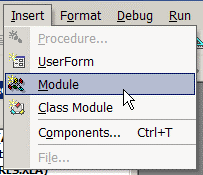
Step 4: Insert a code module from then insert menu

Step 5: Copy the above code to sort the data in excel and paste in the code module which have inserted in the above step

Step 6: Now press F5 to execute the code.

Now you can observe that the Data in Excel sheet is sorted in Ascending/Descending order (as per your requirement and the code used) based on the Column C.

Enable autosort according to a column value for a range of cells.

Sometimes you need to autosort a certain range according to the values in a specific column, You can use the following VBA Macro in the specific excel sheet.

Private Sub Worksheet_Change(ByVal Target As Range)

If Intersect(Target, Range("C3:C20")) Is Nothing Then Exit Sub

Application.EnableEvents = False

Me.Sort.SortFields.Clear

Me.Sort.SortFields.Add Key:=Range("C3:C20"), SortOn:=xlSortOnValues, Order:=xlAscending, DataOption:=xlSortNormal

With Me.Sort

    .SetRange Range("A3:C20")

    .Header = xlGuess

    .MatchCase = False

    .Orientation = xlTopToBottom

    .SortMethod = xlPinYin

    .Apply

End With

Application.EnableEvents = True

End Sub

Values:

C3:C20  -> Column according to which the value will be sorted.

A3:C20 -> Range of cells which will be selected to sort according to the values in C3:C20 column.

VBA Macro to Hide rows depending on Column Value.

Macro to hide rows if the column is blank:

Sub HideRows()
    BeginRow = 1 'Starting row number
    EndRow = 18 ' Ending row number
    ChkCol = 2 'First Column to check for blank values
    ChkCol = 3 'Second Column to check for blank values

    For RowCnt = BeginRow To EndRow
        If Cells(RowCnt, ChkCol).Value = "" Then
            Cells(RowCnt, ChkCol).EntireRow.Hidden = True
        End If
    Next RowCnt
End Sub

For checking only single column for a blank value:

Sub HideRows()
    BeginRow = 1 'Starting row number
    EndRow = 18 ' Ending row number
    ChkCol = 2 'Column to check for blank values

    For RowCnt = BeginRow To EndRow
        If Cells(RowCnt, ChkCol).Value = "" Then
            Cells(RowCnt, ChkCol).EntireRow.Hidden = True
        End If
    Next RowCnt
End Sub

Macro to hide and unhide rows checking the contents of a cell that changes:

You should note that the above macro doesn't unhide any rows, it simply hides them. If you are checking the contents of a cell that can change, you may want to modify the macro a bit so that it will either hide or unhide a row, as necessary. The following changes in the macro will do the trick:

Sub HideRows()
    BeginRow = 1 'Starting row number
    EndRow = 100 ' Ending row number
    ChkCol = 3 'Column to check for blank values

    For RowCnt = BeginRow To EndRow
        If Cells(RowCnt, ChkCol).Value = "" Then
            Cells(RowCnt, ChkCol).EntireRow.Hidden = True
        Else
            Cells(RowCnt, ChkCol).EntireRow.Hidden = False
        End If
    Next RowCnt
End Sub


If you want to include a condition like "less than(<)" and "Greater than(>)" then you can edit the values in the following code of the above macro:

If Cells(RowCnt, ChkCol).Value = "" Then
or
If Cells(RowCnt, ChkCol).Value < 5 Then
or
If Cells(RowCnt, ChkCol).Value > 5 Then

VBA Macro to enable auto hide of blank rows.

The following VBA Macro code will help you in performing auto-hiding blank rows in a specific worksheet.

Sub hideEmptyRows()

Application.ScreenUpdating = False

For i = 3 To 25 'Include the row numbers

  If ActiveSheet.Cells(i, 1) = "" Then

    ActiveSheet.Cells(i, 1).EntireRow.Hidden = True

End If

Next i

Application.ScreenUpdating = True

End Sub

VBA Macro to enable auto filtering in excel.

Sometime, you want to enable the filtering mechanism that you enabled in excel worksheet to be reapplied automatically, then you need to use the following code as Macro which will do it for you:

Private Sub Worksheet_Calculate()

    If Me.FilterMode = True Then

        With Application

            .EnableEvents = False

            .ScreenUpdating = False

        End With

        With ActiveWorkbook

            .CustomViews.Add ViewName:="Mine", RowColSettings:=True

            Me.AutoFilterMode = False

            .CustomViews("Mine").Show

            .CustomViews("Mine").Delete

        End With

        With Application

            .EnableEvents = True

            .ScreenUpdating = True

        End With

    End If

End Sub

Adding VBA Code's to an Excel Workbook

Copy Excel VBA Code to a Regular Module:

Instead of starting from scratch, if you need an Excel macro, you can often find sample code at reputable sites on the internet. To copy that code, and add it to one of your workbooks, follow these steps: 

1. Copy the sample code that you want to use
2. Open the workbook in which you want to add the code
3. Hold the Alt key, and press the F11 key, to open the Visual Basic Editor
4. Choose Insert | Module
5. Where the cursor is flashing, choose Edit | Paste
   

To run the code:

1. On the Excel Ribbon, click the View tab
2. At the far right, click Macros
3. Select a macro in the list, and click the Run button

Copy Excel VBA Code to a Worksheet Module

Another type of Excel code is Event code, which runs automatically when something specific occurs in the workbook. For example, if you enter a number in a cell, or select an entry in a cell's drop down list, the worksheet has been changed. This could trigger the Worksheet_Change event.

Worksheet event code is stored on a worksheet module. To add worksheet event code to your worksheet, do the following:

1. Copy the code that you want to use
2. Select the worksheet in which you the code to run
3. Right click on the sheet tab and click View Code, to open the Visual Basic Editor.

4. Where the cursor is flashing, choose Edit | Paste

Copy Excel VBA Code to a Workbook Module

Another type of code is Workbook Event code, which should be added to the workbook code module:

1. Copy the code that you want to use
2. Select the workbook in which you want to store the code
3. Hold the Alt key, and press the F11 key, to open the Visual Basic Editor
4. In the Project Explorer, find your workbook, and open the list of Microsoft Excel Objects
5. Right-click on the ThisWorkbook object, and choose View Code
6. Where the cursor is flashing, choose Edit | Paste

Copy Excel VBA Code From a Different Workbook

You may find code in a sample workbook online, and decide to add it to one of your workbooks. You can copy all the code in a module by doing the following:

1. Open both workbooks
2. Hold the Alt key, and press the F11 key, to open the Visual Basic Editor
3. In the Project Explorer, find your workbook, and the workbook with the code that you want to copy. The screenshot at the right, the code is in VBACodeCopy.xls and will be copied to MyForm.xlsm
4. In the workbook with the code, click the + sign to view the list of Modules
5. Click on the module that you want to copy, and drag it over the project where you'd like the copy placed.
6. Release the mouse button, and a copy of the module will appear in the workbook.

To run the code:

1. On the Excel Ribbon, click the View tab
2. At the far right, click Macros
3. Select a macro in the list, and click the Run button

Allow Macros to Run in Your Workbook

To use macros in Excel, you might need to enable them when the file opens. If you are using macros for the first time on your current computer, you might also need to adjust the macro security settings.

Follow the instructions below, to make these changes.

Enable Macros When Opening the File

When you open a workbook that contains macros, you might see a security warning, at the top of the worksheet, above the Formula Bar.

1. Click the Options button.
2. Click Enable This Content, to allow the workbook's macros to run, and click OK.

Check Your Macro Security Settings

If you haven't run macros before, you might need to change your macro security level. (You may have to clear this with your IT department.)

1. On the Ribbon, click the Developer tab, and in the Code group, click Macro Security.
2. In the Macro Settings category, under Macro Settings, click Disable all macros with notification
3. Click OK.
4. If you changed the setting, close the workbook, and then reopen it

Run an Excel Macro

After you copy a macro to a regular module, follow the steps below, to run the macro. If the macro does not run, check your macro settings.

To run an Excel macro:

1. Copy the macro code to a regular code module in your file.
2. Then, on the Ribbon's View tab, click the top part of the Macro button, to open the Macro window
3. In the list of macros, click on the macro that you want to run
4. Click the Run button

DATE Function: Print the Last Date of a Month

Syntax:

=DATE (year, month, day)

This function is used to create a valid date from year, month, and day. This will display a serial number that represents a particular date in Excel.

Arguments:

year - The year to use when creating the date.

month - The month to use when creating the date.

day - The day to use when creating the date.

Usage notes:

DATE returns a date serial number. Format the result as a date to display as a date.

If year is between zero and 1900, Excel will add 1900 to the year.

Month can be greater than 12 and less than zero. If month is greater than 12, Excel will add month to the first month in the specified year. If month is less than or equal to zero, Excel will subtract the absolute value of month plus 1 (i.e. ABS(month) + 1) from the first month of the specified year.

Day can be positive or negative. If day is greater than the days in the specified month, Excel will add day to the first day of the specified month. If day is less than or equal to zero, Excel will subtract the absolute value of day plus 1 (i.e. ABS(day) + 1) from the first day of the specified month.

=DATE(year,1,daynum)
Related formulas
Convert date to Julian format
To get a real date from day number, or "nth day of year" you can use the DATE function.

In the example shown, the formula in C5 is:

=DATE(2015,1,B5)
How this formula works

The DATE function build dates from separate year, month, and day values. One of it's tricks is the ability to roll forward to correct dates when given days and months that are "out of range".

For example, DATE returns April 9, 2016 with the following arguments:

=DATE(2016,1,100)
There is no 100th day in January, so DATE simple moves forward 100 days from January 1 and figures returns the correct date.

The formula on this page takes advantage of this behavior. The year assumed to be 2015 in this case, so 2015 is hard-coded for year, and 1 is used for month. The day value comes from column B, and the DATE function calculates the date as explained above.

Extracting a year value from a Julian date

If you have a date in a Julian format, for example, 10015, where the format is "dddyy", you can adapt the formula as follows:

=DATE(RIGHT(A1,2),1,LEFT(A1,3))

Here, we use RIGHT to extract the 2 characters from the right for year, and LEFT to extract 3 characters from the left for day. Month is supplied as 1, like the first example.

For example: 

Find the last date of a month:

=DATE(YEAR(date),MONTH(date)+1,0)

=DATE($E$1,MONTH(DATEVALUE($D$1&" 1"))+1,0)

$E$1  has the Year value.

$D$1 has the Month Name.

For more info regarding YEAR and DATEVALUE functions please check YEAR and DATEVALUE

YEAR Function and it's usage.

Syntax: 

=YEAR (date)

This function will help you get the year from a date. It will display a number representing year.

Arguments: 
date - A date from which to extract the year.

Usage notes: 
date - date must be a valid Excel date in serial number format. For example, the date Jan 1, 2000 is equal to the serial number 32526 in Excel

Excel only handles dates after 1/1/1900.

=YEAR(date)
If you need to extract the year from a date, you can use the YEAR function. In the generic form of the formula above, the date  must be in a form that Excel recognizes as a valid date.

Here's how the formula works:

The YEAR function takes just one argument, the date from which you want to extract the year. In the example, the formula is:

=YEAR(B4)

B4 contains a date value for July 7, 2016. The YEAR function returns the number 2016 representing the year of the date.

Note that you can use YEAR to extract the year from a day entered as text:

=YEAR("1/5/2016")

However, using text for dates can cause unpredictable results on computers using different regional date settings. In general it's better (and more flexible) to supply an address to a cell that already contains a valid date.

DATEVALUE Function.

Syntax:

=DATEVALUE (date_text)

This displays a serial number that represents a particular date in Excel. It converts a date in text format to a valid date.

Arguments:
date_text - A valid date in text format.

Usage notes:
If date_text is a cell address, the value of the cell must be text. If date_text is entered directly into the formula it must be enclosed in quotes.

Will return a #VALUE error if date_text refers to a cell that does not contain a date formatted as text.

VLOOKUP Function: Lookup specific value in a column and pull the data corresponding to it.

Syntax:

=VLOOKUP (value, table, col_index, [range_lookup])

Arguments:

value - The value to look for in the first column of a table.

table - The table from which to retrieve a value.

col_index - The column in the table from which to retrieve a value.

range_lookup - [optional] TRUE = approximate match (default). FALSE = exact match.

Usage notes:

VLOOKUP searches for a value in the first column of a table. At the match row, it retrieves a value from the specified column.

Use VLOOKUP when lookup values are located in the first column of a table with information organized vertically. Use HLOOKUP when lookup values are located in the first row of a table, and each "record" appears in a new column.

• Range_lookup controls whether value needs to match exactly or not. The default is TRUE = allow non-exact match.
• Set range_lookup to FALSE to require an exact match and TRUE to allow a non-exact match.
• If range_lookup is TRUE (the default setting), a non-exact match will cause the VLOOKUP function to match the nearest value in the table that is still less than value.
• When range_lookup is omitted, the VLOOKUP function will allow a non-exact match, but it will use an exact match if one exists.
• If range_lookup is TRUE (the default setting) make sure that lookup values in the first row of the table are sorted in ascending order. Otherwise, VLOOKUP may return an incorrect or unexpected value.
• If range_lookup is FALSE (require exact match), values in the first column of table do not need to be sorted.

For Example:

Lookup specific value in a column and pull the data corresponding to it.

=VLOOKUP($A3,'Sheet_Name'!$A:$ZZ,4,0)

value - $A3 (The Value in A3, $ means the column A will not change when we drag the formula to other cells)

table - 'Sheet_Name'!$A:$ZZ

col_index - Column number 4.

range_lookup - 0 means FALSE, which means exact match.

Lookup specific value in a column and pull the data corresponding to it except the word 'Tickets with QA score'(IF Function with Vlookup Function):

=IF(VLOOKUP($A3,'Sheet_Name'!$A$1:$ZZ$500,4,0)="Tickets with QA score","",(VLOOKUP($A3,'Sheet_Name'!$A$1:$ZZ$500,4,0)))

For more info regarding IF function please check IF.

Business Automation: Find subscriptions which are not Auto-renewed.

Tested on Version: Business Automation 6.x

In-order to find the subscription's with auto-renewal enabled and expiration date = today (or in past) and are not auto-renewed, you can run the following query in Odin Business Automation Database:

pba=> SELECT s."subscriptionID", s."PlanID", s."AccountID", a."VendorAccountID" AS "Reseller ID", s."Status", s."ServStatus", s."renewalOrderOrderID" AS "Renewal Order ID", so."OrderStatusID", s."ExpirationDate"::ABSTIME::DATE,s."ShutdownDate"::ABSTIME::DATE, s."TerminateDate"::ABSTIME::DATE FROM "Subscription" s INNER JOIN "Account" a ON (s."AccountID" = a."AccountID") LEFT JOIN "SalesOrder" so ON (s."renewalOrderOrderID" IS NOT NULL AND s."renewalOrderOrderID" = so."OrderID") WHERE s."Status" IN (30) AND s."IsAutoRenew" = 1 AND s."ExpirationDate"::ABSTIME <= now()::ABSTIME::DATE ORDER BY s."subscriptionID";


To count the number of subscriptions which are not auto-renewed:

pba=> SELECT count(*) FROM "Subscription" as s INNER JOIN "Account" a ON (s."AccountID" = a."AccountID") LEFT JOIN "SalesOrder" so ON (s."renewalOrderOrderID" IS NOT NULL AND s."renewalOrderOrderID" = so."OrderID") WHERE s."Status" IN (30) AND s."IsAutoRenew" = 1 AND s."ExpirationDate"::ABSTIME <= now()::ABSTIME::DATE;
 count
-------
     0
(1 row)

pba=>

IF Function: Copy data from another column and eliminate 0 values for blank cells and the word "grand total"

Syntax:

=IF (logical_test, [value_if_true], [value_if_false])

Arguments:
logical_test - A value or logical expression that can be evaluated as TRUE or FALSE.
value_if_true - [optional] The value to return when logical_test evaluates to TRUE.
value_if_false - [optional] The value to return when logical_test evaluates to FALSE.

Usage notes: 
Use the IF function to test for or evaluate certain conditions, and then react differently depending on whether the test was TRUE or FALSE.

For example, let's say you want to assign either "Pass" or "Fail" to students based on a test score. In that case, you need to test the sore itself (for each student) and then return either "Pass" or "Fail".

If you had a score in cell C6, and you wanted to test this score to see if is at least 70, you would use this:

C6>=70
This translates as "C6 contains a value greater than or equal to 70". It will either be TRUE or FALSE, depending on the value in C6. You then supply a value that the IF function should return if the test is TRUE, and a value to use if the test is FALSE.

Putting it all together, you would use this formula:

=IF(C6>=70, "Pass", "Fail")
This is the formula that appears D6 in the example shown. When it is copied down the column, it will test every score and return the correct result.

Nested IF statements:
You may here the term "Nested IF" or "Nested IF statement". This refers to using more than one IF function so that you can test for more conditions and return more possible results. Each IF statement needs to be carefully "nested" inside another so that the logic is correct.

For example, the following formula can be used to assign an grade rather than a pass / fail result:

=IF(C6<70,"F",IF(C6<75,"D",IF(C6<85,"C",IF(C6<95,"B","A"))))
Up to 64 IF functions can be nested. However, in general, you should consider other functions, like VLOOKUP or HLOOKUP for more complex scenarios, because they can handle more conditions in much more streamlined fashion.

Logical operators:
When you are constructing a test with IF, you can use any of the following logical operators:

Comparison operator	Meaning	Example
=	equal to	A1=D1
>	greater than	A1>D1
>=	greater than or equal to	A1>=D1
<	less than	A1
<=	less than or equal to	A1<=D1
<>	not equal to	A1<>D1

Notes:

• If any of the arguments to IF are supplied as arrays, the IF function will evaluate every element of the array.
• To count things conditionally, use the COUNTIF or the COUNTIFS functions.
• To sum things conditionally, use the SUMIF or the SUMIFS functions.

For Example to Copy data from another column and eliminate 0 values for blank cells and the word grand total:

=IF(IF('Sheet_Name'!$A8="","",'Sheet_Name'!$A8)="Grand Total","",(IF('Sheet_Name'!$A8="","",'Sheet_Name'!$A8)))

logical_test - IF('Sheet_Name'!$A8="","",'Sheet_Name'!$A8)="Grand Total"
value_if_true - "" (It means print Blank)
value_if_false - (IF('Sheet_Name'!$A8="","",'Sheet_Name'!$A8)

INDEX Function: Print the value with intersection of row and column:

Syntax: 

=INDEX (array, row_num, [col_num], [area_num])

Arguments: 

array - A range of cells, or an array constant.

row_num - The row position in the reference or array.

col_num - [optional] The column position in the reference or array.

area_num - [optional] The range in reference that should be used.

Usage notes: 

Use the INDEX function to get a value from a list or table based on its location.
For example, the formula =INDEX(A1:B5,3,3) will return the value at the address B3.

The INDEX function has two forms: array and reference.

• Array form:

In the array form of INDEX, the first parameter is array, which is supplied as a range of cells or an array constant. The syntax for the array form of INDEX is:

INDEX (array, row_num, [col_num])
If both row_num and col_num are supplied, INDEX returns the value in the cell at the intersection of row_num and col_num.
If your row_num is set to zero, INDEX returns an array of values for the entire row. To use these array values, enter the INDEX function as an array formula in horizontal range.
If you col_num is set to zero, INDEX returns an array of values for the entire column. To use these array values, enter the INDEX function as an array formula in vertical range. 

• Reference form

In the array form of INDEX, the first parameter is reference, which is supplied as a reference to one or more cell ranges. The syntax for the reference form of INDEX is:

       INDEX (reference, row_num, [col_num], [area_num])
The reference form of INDEX returns the reference of the cell at the intersection row_num and col_num.

If reference is supplied as multiple ranges,  area_num indicates which range to use.

area_sum is supplied as a number.
For example, in the formula =INDEX((A1:C5,A7:C10),2,2,2),area_num is supplied as 2, which refers to the range A7:C10.

Examples:

1. Print the value which is existing in the intersection of row 84 and in column 13:

=INDEX('Sheet_Name'!1:1048576,84,13)

array - 'Sheet_Name'!1:1048576  (Check in complete sheet Sheet_Name)

row_num - 84

col_num - 13

2. Print the data present in intersection of the column and row values (data retrieved from above formulas):

=INDEX('Sheet_Name'!1:1048576,MATCH("Grand Total",'Sheet_Name'!$A:$A,0),MATCH(A7,'Sheet_Name'!A8:Z8,0))

array - 'Sheet_Name'!1:1048576  (Check in complete sheet Sheet_Name)

row_num - MATCH("Grand Total",'Sheet_Name'!$A:$A,0)

col_num - MATCH(A7,'Sheet_Name'!A8:Z8,0)

For more info regarding MATCH function: MATCH

Search in a row and Find Column number matching from the data in a column:

In-order to search a row and find the column number which is matching the data in the column you can use the following formula: 

=MATCH(A7,'Sheet_Name'!A8:Z8,0)

lookup_value - A7 (Value in column A7 in the same sheet)

lookup_array - 'Sheet_Name'!A8:Z8 (Check row 8 in worksheet Sheet_Name)

match_type - 0

For detailed info regarding MATCH formula, please look MATCH.

MATCH Function - Formula to find the row number where "Grand Total" is existing:

Syntax:

=MATCH (lookup_value, lookup_array, [match_type])

Arguments: 

lookup_value - The value to match in lookup_array.

lookup_array - A range of cells or an array reference.

match_type - [optional] How to match, specified as -1, 0, or 1. Default is 1.

Usage notes: 

Use the MATCH function to get the relative position of an item in an array. Match offers several different matching modes, which makes it more flexible than other lookup functions. Used together with INDEX, MATCH can retrieve the value at the matched position.

Match type information:

• If match_type is 1, MATCH finds the largest value that is less than or equal to lookup_value. The lookup_array must be sorted in ascending order.
• If match_type is 0, MATCH finds the first value exactly equal to lookup_value. lookup_array does not need to be sorted.
• If match_type is -1, MATCH finds the smallest value that is greater than or equal to lookup_value. The lookup_array must be sorted in descending order.
• If match_type is omitted, it is assumed to be 1.
• Note: All match types will find an exact match.

Notes:

• Match is not case-sensitive.
• Match returns the #N/A error if no match is found
• The argument lookup_array must be placed in descending order: TRUE, FALSE, Z-A,...2, 1, 0, -1, -2,..., and so on.
• If match_type is 0 and lookup_value is text, the wildcard characters question mark (?) and asterisk (*) can be used in lookup_value. 
• If match_type is 0 and lookup_value is text, lookup_value can contain the wildcard characters asterisk (*) and question mark (?). An asterisk matches any sequence of characters; a question mark matches any single character.

Formula to find the row number where "Grand Total" is existing:

=MATCH("Grand Total",'Sheet_Name'!$A:$A,0)

lookup_value - "Grand Total"

lookup_array - 'Sheet_Name'!$A:$A (Check Column A in worksheet Sheet_Name)

match_type - 0